Brain-Inspired Approaches to Speech Detection

This blog post ssumes you’ve completed the LibriBrain tutorials and are familiar with the baseline models.

The tutorial models make specific assumptions—like focusing on only 23 (out of 306) sensors around the superior temporal gyrus (STG). But are these assumptions optimal? And what else might we learn from how the brain actually processes speech in order to design clever decoding models? In this blog, we discuss some of what we know from neuroscience and how you might use this information to improve your competition submissions.

Why STG Matters (But Isn’t Everything)

#

The 23 sensors selected in the tutorial aren’t random. In the LibriBrain dataset paper (Özdogan et al., 2025), we systematically analysed signal quality across all 306 MEG sensors and found the strongest speech-related activity concentrated in bilateral STG regions. The result of this data-driven approach is the 23 sensors you see in the tutorial (note that each of the code blocks below is scrollable left-to-right):

SENSORS_SPEECH_MASK = [18, 20, 22, 23, 45, 120, 138, 140, 142, 143, 145, 146, 147, 149, 175, 176, 177, 179, 180, 198, 271, 272, 275]

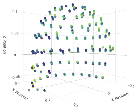
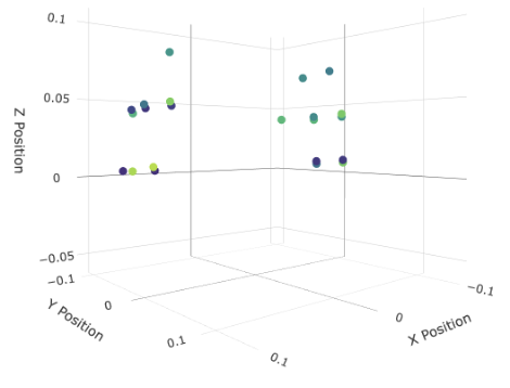
Left: All MEG sensors in the LibriBrain dataset, as shown with the interactive viewer (see Speech Detection Colab Tutorial or the similar interactive visualisation below). Right: the sensors used in the mask. To create your own mask, the spatial coordinates for each sensor are on the competition website here.

The 23 channels used for the speech detection reference model were selected based on the most robust amplitude, phase and power modulations observed in our 50+ hour dataset:

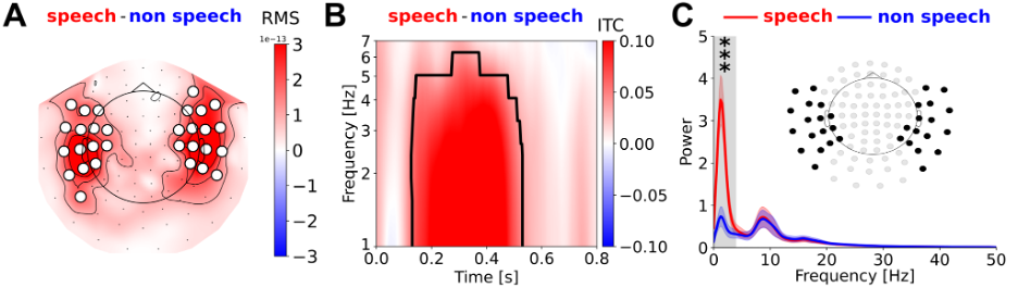
Sensors clustered around the STG, topographic map from Özdogan et al. 2025 (Figure 9).

Topographic maps, like that shown here (in panel A), provide a top-down view of a cartoon head (black circle) with the nose on top (black triangle). This means that the left and right sides of the head correspond to your left and right. Despite appearances, it does not mean that the sensors (filled white circles) are positioned outside of the head. By convention, the correct way to read topographic maps like this is to imagine that the sensors wrap around the side of the head. Likewise, the brain activity that is represented in shades of red and demarcated by contours can be seen largely around the left and right sides of the head, which is where we would expect to find it from neuroscience.

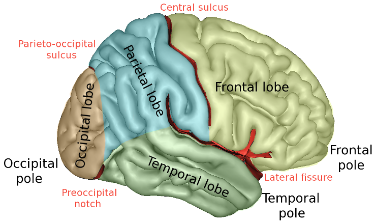
The four lobes of the brain (frontal, temporal, parietal, and occipital), with other key landmarks like the lateral fissure, central sulcus, and temporal pole (image from Wikipedia).

There are three major ridges (or gyri) along the temporal lobe, if you move your eyes from right to left from the temporal pole. The upper-most ridge (or gyrus) is the STG. Its role in auditory (and speech) processing makes sense given its proximity to the primary auditory cortex (A1), which is located on the upper surface of the temporal lobe inside the lateral fissure.

But this doesn’t mean there aren’t other sensor configurations worth exploring.

Neuroscientific studies of speech detection have not only found signals around the STG (e.g. Hamilton et al. 2018) but also show brain activity while people listen to speech in areas around the central sulcus, between the frontal and parietal lobes (e.g. Cheung et al. 2016). In their seminal study of speech decoding in paralysed individuals, Moses et al. (2021) further showed that attempted speech could be decoded from electrodes placed on the surface of the brain around the central sulcus. Here’s a guess of which MEG sensors might correspond with this:

SENSORS_CENTRAL_SULCUS_MASK = [18, 19, 20, 42, 43, 44, 45, 46, 47, 72, 73, 74, 75, 76, 77, 78, 79, 80, 81, 82, 83, 120, 121, 122, 123, 124, 125, 145, 146, 147, 148, 149, 201, 202, 203, 246, 247, 248]

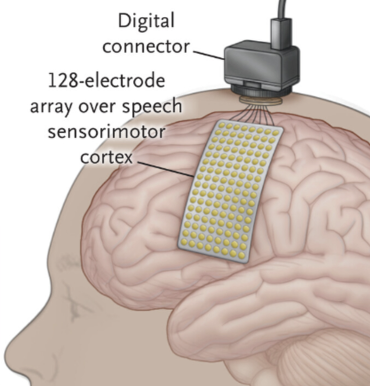
Location of sensors used for speech detection from Moses et al. 2021 (Figure 1).

In another study of speech detection, Kurteff et al. (2024) identified yet another brain region: the insula. Located more deeply in the brain, MEG signals for the insula might be expected to show up across a broad range of sensors. In any case, there is information about speech detection in many parts of the brain. Decoding offers a chance to study, empirically, which sensors are best for predicting speech and non-speech across the whole brain.

Posterior and Anterior Divisions within the STG

#

Neuroscience can also tell us something about how speech is detected in the brain. Using invasive electrocorticography (ECoG), Hamilton et al. (2018) make a distinction between two parts of the STG:

• Posterior STG: Responds strongly to acoustic onsets—the transitions from silence to speech
• Anterior STG: Shows sustained responses throughout speech events

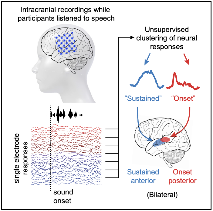
Figure reproduced from Hamilton et al. 2018 (graphical abstract).

This spatial organisation suggests that even within the tutorial’s 23-sensor selection, different sensors might be doing different jobs: some might be better for detecting speech boundaries; others for sustained content processing. Using the highly sophisticated method of “eyeballing” the figure from the Hamilton et al. paper, here’s an initial guess at picking sensors which uses ~35% of the posterior STG for onset detection:

SENSORS_STG_POSTERIOR = [12, 13, 14, 18, 19, 20, 21, 22, 23, 141, 142, 143, 144, 145, 146, 147, 148, 149, 174, 175, 176, 177, 178, 179, 180, 181, 182, 198, 199, 200, 249, 250, 251, 270, 271, 272, 273, 274, 275, 279, 280, 281]

SENSORS_STG_ANTERIOR = [15, 16, 17, 18, 19, 20, 21, 22, 23, 45, 46, 47, 120, 121, 122, 138, 139, 140, 144, 145, 146, 147, 148, 149]

This is a good start but it is not the only way we can take advantage of these insights. What else might we do?

Relabelling events to add classes: Another idea for taking advantage of the result from Hamilton et al. (2018) would be to relabel the target events to distinguish “onset of speech” from “sustained speech”. Concretely, what do we mean?

In the LibriBrain dataset, speech detection is formulated as simple binary classification, with “speech” labelled as “1” and “non-speech” labelled as “0”. One way to distinguish onset and sustained speech would be to introduce a third label for “onset speech”, relabelling the first n speech labels after an onset as “2” instead of “1”.

To illustrate for n=3, you would replace an original sequence of labels [0, 0, 0, 0, 1, 1, 1, 1] with a new sequence [0, 0, 0, 0, 2, 2, 2, 1]. The choice of n here was illustrative. A more realistic prior for n might range from around 33 to 36 labels, given that speech onset events have durations of 138 ± 5 ms (Hamilton et al. 2018) and the sample rate of the LibriBrain data is 250 Hz (4 ms per sample).

Whatever n you pick, a model trained on these labels should implicitly learn different representations for the events “onset speech” and “sustained speech”, rather than being forced to learn a unified label for both. Finally, before submitting to the EvalAI platform, simply replace all predicted “2” labels with “1”, making the labels binary again.

What about other relabelling schemes? What about adding a “speech offset” class? While we do not know of any neuroscientific evidence showing the brain’s preference for a “speech offset” event, which would represent the transition from speech to non-speech, the decoding framework provides a way of learning new things.

Whatever works to improve speech detection in the LibriBrain dataset provides evidence of how speech is organised in the brain. So, by doing good machine learning, you could make a novel contribution to neuroscience.

Target smoothing/interpolation: Another assumption of the default labelling scheme is that transitions between speech and non-speech are almost instantaneous, occurring within the 4 ms represented by the 250 Hz sampling rate.

If state transitions in the brain are slower, then it could make sense to smooth (or interpolate) the target labels. For example, a sequence like [0, 0, 0, 1, 1, 1] might become [0, 0.2, 0.4, 0.6, 0.8, 1]. This assumes linear interpolation, but of course there are lots of non-linear alternatives such as sigmoid functions with steeper or more gradual transitions.

Smoothing might also make sense if there is label noise (uncertainty in the event boundaries).

Modelling conduction delays: How confident are we about the precision of changes between speech detection labels?

While we’ve gone beyond what is typical for methodological rigour and quality control in neural datasets, as reflected empirically by the results of comparative studies such as Jayalath et al. 2025, this might be a good opportunity to explain how speech labels were assigned in the LibriBrain dataset.

The audio played to the subject in the MEG scanner went through multiple checks to produce the event files. First, we used voice activity detection (VAD) to automatically segment audio into speech and non-speech. This used an amplitude threshold together with a set of carefully tuned heuristics (e.g. a minimal duration for speech events). But it was still not perfect. For instance, quiet sounds (such as plosives like /p, t, k/) might be missed at the beginning of utterances. We therefore took the extraordinary step of manually checking (and correcting) all of the events—to give a sense of scale, this took hundreds of hours of manual labour to complete.

In line with the “minimal preprocessing” philosophy of the LibriBrain dataset, no temporal offsets were added to the speech labels. In other words, the speech and non-speech labels from the audio were taken directly as labels for the brain. Although we know that there are conduction delays between the ear and cortex, these delays are not constant across the whole brain. In other words, there is not a single temporal offset from the ear to all parts of the brain. Furthermore, even for specific brain regions, we might not be certain about the precise delay. Ultimately, any explicit offset or set of offsets that we add to the data might introduce errors. We have therefore chosen to trust users to explicitly account for conduction delays.

So what should you do? Perhaps the most straightforward advice would be to investigate models that are either invariant to small temporal offsets or that explicitly learn offsets.

Methods that make models less sensitive to exact timing include target smoothing (discussed above), temporal pooling, and data augmentation strategies that add temporal jitter. Some of these are used in the speech detection reference model (Landau et al. 2025a,b, where the latter is our dedicated blog post on the reference model). You might also tune the receptive field of architectures that use strided/dilated convolutions. Various model architectures will learn offsets such as transformers, through the use of attention mechanisms.

For anyone looking for a deeper dive into the neurobiology of audition and of speech comprehension, we heartily recommend Schnupp et al. (2011) and Parker Jones & Schnupp (2021)—the former is the standard Auditory Neuroscience textbook, whereas the latter is a more recent update of the field emphasising new advances in our understanding of speech.

Interactive 3D Sensor Visualisation

#

Explore the MEG sensor positions and the different sensor masks discussed in this blog post. Use the controls below to visualise how different brain regions map to MEG sensors. Note: The masks provided are our best initial guess. We highly recommend that you to play around with the data yourself to find out what works for you.

Ready to implement these ideas? Check out the LibriBrain competition tutorials and join the discussion on Discord. The competition runs through September 2025, with both Standard and Extended tracks to accommodate different resource levels.

Key References

#

Broderick, M. P., et al. (2018). Electrophysiological correlates of semantic dissimilarity reflect the comprehension of natural, narrative speech. Current Biology, 28, 803-809.

Cheung, C., Hamilton, L. S., Johnson, K., & Chang, E. F. (2016). The auditory representation of speech sounds in human motor cortex. Elife,5, e12577. Crosse, M. J., et al. (2016). The multivariate temporal response function (mTRF) toolbox. Frontiers in Human Neuroscience, 10, 604. Di Liberto, G. M., et al. (2015). Low-frequency cortical entrainment to speech reflects phoneme-level processing. Current Biology, 25, 2457-2465.

Ding, N., & Simon, J. Z. (2014). Cortical entrainment to continuous speech: functional roles and interpretations. Frontiers in human neuroscience, 8, 311.

Giraud, A. L., & Poeppel, D. (2012). Cortical oscillations and speech processing: emerging computational principles and operations. Nature neuroscience, 15(4), 511-517.

Hamilton, L. S., et al. (2018). A spatial map of onset and sustained responses to speech in the human superior temporal gyrus. Current Biology, 28, 1860-1871.

Jayalath, D., Landau, G., & Parker Jones, O. (2025). Unlocking non-invasive brain-to-text. ICML Workshop on Generative AI and Biology.

Kurteff, G. L., et al. (2024). Spatiotemporal mapping of auditory onsets during speech production. Journal of Neuroscience, 44(47), e1109242024.

Landau, G., Özdogan, M., Elvers, G., Mantegna, F., Somaiya, P., Jayalath, D., Kurth, L., Kwon, T., Shillingford, B., Farquhar, G., Jiang, M., Jerbi, K., Abdelhedi, H., Mantilla Ramos, Y., Gulcehre, C., Woolrich, M., Voets, N., & Parker Jones, O. (2025a). The 2025 PNPL competition: Speech detection and phoneme classification in the LibriBrain dataset. NeurIPS Competition Track.

Landau, G., Elvers, G., Özdogan, M., & Parker Jones, O. (2025b). The speech detection task and the reference model [Blog post]. Neural Processing Lab. https://neural-processing-lab.github.io/2025-libribrain-competition/blog/speech-detection-reference-model

Luo, H., & Poeppel, D. (2007). Phase patterns of neuronal responses reliably discriminate speech in human auditory cortex. Neuron, 54(6), 1001-1010.

Özdogan, M., Landau, G., Elvers, G., Jayalath, D., Somaiya, P., Mantegna, F., Woolrich, M., & Parker Jones, O. (2025). LibriBrain: Over 50 hours of within-subject MEG to improve speech decoding methods at scale. arXiv preprint.

Parker Jones, O., & Schnupp, J. W. H. (2021). How does the brain represent speech? In J. S. Pardo, L. C. Nygaard, R. E. Remez, & D. B. Pisoni (eds.), The handbook of speech perception (2nd ed., Chapter 3). Wiley.

Peelle, J. E., & Davis, M. H. (2012). Neural oscillations carry speech rhythm through to comprehension. Frontiers in psychology, 3, 320.

Schnupp, J. W. H., Nelken, I., & King, A. J. (2011). Auditory neuroscience: Making sense of sound. The MIT Press.

Citation

#

@misc{pnpl_blog2025brainInspiredSpeechDetection,
  title={Brain-Inspired Approaches to Speech Detection},
  author={Mantegna, Francesco and Elvers, Gereon and Parker Jones, Oiwi},
  year={2025},
  url={https://neural-processing-lab.github.io/2025-libribrain-competition/blog/brain-inspired-approaches-speech-detection},
  note={Blog post}
}